6-Axis Force Sensor Analog Output Acquisition

1. What the sizing results can help you decide

Engineering review: 2 November 2026. All examples are calculations, not measured results or approved product configurations. The report below uses fixed illustrative examples, independent of your submitted tool inputs.

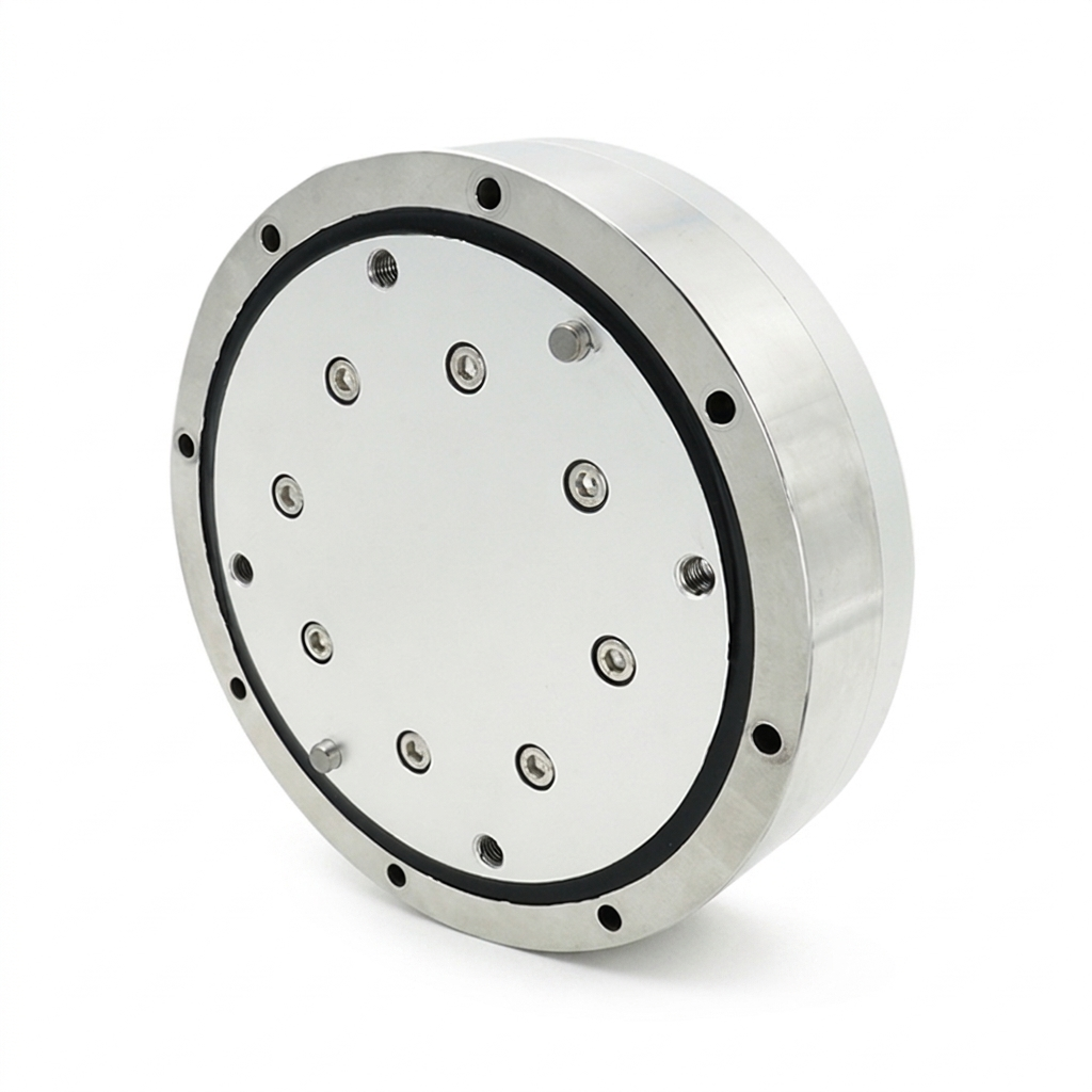
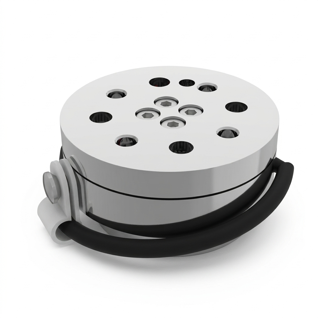
Use the package references to discuss connector access, cable routing and the location of signal conditioning. They illustrate geometry only; an exterior photo cannot establish raw-bridge output, pinout, ADC architecture or a calibration rating.

Request the electrical block diagram and serial-linked calibration record before choosing between a remote DAQ and near-sensor electronics.

↗

↗

2. Model, units and limits

The model contains six identical full bridges with one raw differential channel per bridge. Excitation is a DC magnitude, sensitivity is the one-sided rated bridge output in mV/V, ADC range is a symmetric differential peak limit, and sample rate means frames per second with one sample per channel per frame. Individual bridges may respond to multiple mechanical axes; raw channels are not automatically Fx through Mz.

This is a baseband planning model. It excludes bridge imbalance, unequal sensitivities, AFE offset/common-mode limits, connector resistance, wire heating, source impedance, actual filter response and the calibration matrix. A conditioned voltage-output sensor needs its own scaling model. For circuit architectures and constraints see the TI bridge measurement guide.

The 0.5% cable-loss, 500 mW heating and 10× sampling-ratio flags are editorial review triggers. They are not manufacturer ratings or universal acceptance criteria. Every configuration retains unverified hardware requirements.

3. Excitation: calculate power, measure thermal behavior

Use the voltage approved for the actual bridge and electronics. Raising excitation increases signal linearly and dissipation quadratically at fixed resistance. The examples below assume ideal voltage at each of six 350 Ω bridges; power excludes excitation-wire losses. A compact sensor and a large balance can have very different thermal resistance at the same power.

Do not infer a safe excitation limit from this table. Ask for maximum excitation, input resistance tolerance and zero/span temperature coefficients. Record cold-start zero and ambient temperature with the intended mounting, then choose a warm-up/tare procedure from the observed settling. Do not add interface paste or insulating spacers without checking mounting and calibration requirements.

4. Gain, common mode and overload are separate checks

For the default 5 V, 1.2 mV/V bridge, nominal full-scale output is 6 mV. Mapping that through a 1.5× allowance into ±2.5 V gives G = (2.5/1.5)/0.006 = 277.8×. Nominal ADC peak is 1.667 V, leaving 0.833 V, or 33.3% of the positive peak range. These numbers do not account for bridge zero offset or combined loading.

Check both polarities of every raw channel under maximum expected tool tare, acceleration and applied wrench. A digital tare after the ADC cannot recover clipping that happened earlier. Confirm amplifier input common mode, output swing, supplies, gain-bandwidth and settling before interpreting the arithmetic gain as realizable.

The generic ±2.5 V calculator setting is not an ADS131M06 preset. That device is a six-channel simultaneous 24-bit converter with its own reference, PGA and input constraints; inspect those conditions before connecting a bridge or external amplifier. No compatibility test is claimed. TI ADS131M06 datasheet.

5. Sampling: bandwidth first, then channel alignment

For the selected baseband model, the highest relevant component must be strictly below fs/2. Equality is rejected because arbitrary phase cannot be recovered reliably at the boundary. A real anti-alias filter also needs transition bandwidth; the inequality alone does not establish adequate attenuation. ADI MT-002 sampling tutorial.

A 1 kHz frame rate means 6,000 conversions/s in this uniform-scan example, giving 833.3 µs endpoint skew and 15° at 50 Hz. A burst scan can be much shorter; delta-sigma channel switching can instead require additional settling. Use actual device timing. The phase value alone cannot predict off-axis force or controller stability without signal amplitudes, matrix coefficients and the full control-loop model.

Simultaneous acquisition reduces one source of mismatch; common filter configuration and clocking still matter. Multiplexing may be acceptable for slow signals with a proven error budget. Do not treat it as universally invalid or simultaneous sampling as zero-error measurement.

Choose filters by passband amplitude error, stopband rejection, group delay and settling. Bessel, Butterworth and sinc filters offer different tradeoffs; neither a filter family nor a nominal sample rate guarantees contact stability. Evaluate analog and converter digital filters together, then measure end-to-end latency under load.

6. Cable loss: declare the current path

A 5 m harness at the assumed 0.134 Ω/m has a 1.34 Ω round-trip excitation resistance. That produces about 0.38% uncompensated drop for one 350 Ω load, versus about 2.25% when six such bridges share one pair. The wiring drawing determines which model applies.

Six-wire sensing can feed a voltage regulator or the measurement reference; these are distinct implementations. The tool specifically assumes active regulation. Confirm source compliance/current and sense-loop behavior, then measure residual error. A remote sense pair does not imply unlimited cable length or a measured 0.00% loss. NI remote sensing manual.

Ratiometric cancellation assumes the reference follows the actual bridge excitation with compatible scaling and dynamics. An independent reference retains excitation drift as a gain term. Because drift/noise transfer data are not inputs here, the reference selector changes the review advice rather than inventing a numerical improvement. TI bridge measurement guide.

7. Noise: an ideal estimate has a clear boundary

The calculator uses ebridge = √(4kTRB), T = 300 K and ideal brick-wall B = fs/2. For equal full-bridge arms and a low-impedance excitation source, differential output resistance equals the arm resistance. Real excitation impedance and bridge topology can change this. At the default 350 Ω and 500 Hz bandwidth, the estimate is 0.054 µV RMS at the bridge.

For a bipolar ±A ADC, code step q = 2A/2ᴺ and ideal quantization RMS is q/√12. The displayed ideal SNR is 20 log₁₀[(Vpeak/√2)/√((G·ebridge)² + q²/12)], using a nominal-load sine and the modeled cable voltage. Quantization noise is a statistical idealization; a real converter must be characterized. ADI ADC noise definitions.

To compare two chains, capture equal-duration unloaded data at the same bandwidth and temperature. Report raw and decoupled RMS noise, peak-to-peak behavior, drift and filtering separately. A 24-bit data word does not establish 24 effective bits or any specific force resolution.

8. Matrix processing, units and numerical checks

Apply the supplied calibration convention: W = C(S − S₀). S may be volts, mV/V or ADC codes depending on the calibration record; C must match that convention. Preserve serial number, revision, channel order, sign, coordinate frame and force/torque units. Changing excitation or gain may invalidate a voltage-based matrix.

A direct 6×6 matrix-vector product requires 36 multiplies and 30 additions per frame, excluding zero subtraction, filtering and diagnostics. At 1 kHz this is 66,000 arithmetic operations/s and a 1,000 µs frame period. These counts do not determine MCU execution time: compiler, clock, arithmetic, memory access and interrupt load must be specified and measured.

If output torques are divided by a declared characteristic length L, define D = diag(1,1,1,1/L,1/L,1/L). Since the output is W = CS, normalized output is Wn = DW and Cn = DC. Scaling acts on output rows. Changing input normalization requires a separate right-side transform. Declare both scales before comparing condition numbers; no universal threshold certifies sensor geometry.

For a linear model, output noise covariance is ΣW = CΣSCᵀ. This directly connects measured channel noise to output uncertainty. A small condition number alone does not set absolute noise gain, residual crosstalk or accuracy; retain calibration residuals and uncertainty evidence.

9. Four reproducible planning examples

These are hypothetical input sets. Each link loads the exact preset into the calculator; all outcomes below are arithmetic or required verification, not observed device performance.

10. Architecture choices and cost risks

Quotes must include the sensor, conditioning, DAQ channels, excitation supply, cable/connectors, mounting, calibration, firmware and acceptance tests. Prices and lead times are unknown here. A lower converter price may increase integration and recalibration work; compare the complete accepted chain.

Misuse risk: electrical headroom does not protect the flexure from overload. Scenario mismatch: a static fixture and a contact controller need different timing/error budgets. EMI risk: grounding and shield terminations depend on chassis bonding, frequency and installation; follow the equipment wiring instructions and test the installed system rather than imposing a universal single-end shield rule.

For existing interface families start with the interface overview. All HexaForce analog features and compatibility remain configuration targets until confirmed in writing; this page does not establish a tested SKU or driver.

11. Repeatable bench acceptance checklist

This is an original planning protocol. Agree measurable limits, test equipment uncertainty and allowable loads before testing; no universal release thresholds are imposed. Retain the actual configuration, raw logs, scripts and pass/fail evidence.

1. Freeze the chain: record sensor serial/calibration revision, bridge ratings, pinout, gain, ADC range/rate/filter, reference topology, cable drawing, firmware and intended wrench frame. Missing evidence means the review remains open.
2. Confirm wiring and excitation: follow the approved pinout, check unpowered resistances using the supplier’s method, then measure bridge-end voltage and current under load. Test the complete harness and source compliance; do not infer regulated voltage from a software setting.
3. Characterize offsets and noise: log unloaded raw channels and ambient temperature through warm-up. Report bandwidth, RMS, peak-to-peak and drift separately; use the measured settling to define when tare is allowed.
4. Check channel timing: review ADC and filter timing. Apply a safe, synchronized electrical input using suitable test fixtures and compare channel phase with sufficient bandwidth and uncertainty. Frame timestamps alone cannot certify nanosecond skew.
5. Check raw electrical headroom: exercise an approved load/tool trajectory within mechanical limits, retain both peak polarities for all channels and compare to AFE/ADC rails. Do not rely on zeroed or decoupled readings to detect clipping.
6. Verify mechanical conversion: apply traceable loads within the approved envelope and compare all six outputs, units and signs. Specify off-axis residuals against each relevant rated axis; check combined loads where required. Electrical shunt tests do not replace mechanical calibration.
7. Measure system timing and environment: log worst-case acquisition-to-host age, jitter, dropped frames and behavior with drives active. Use the agreed uncertainty and control requirements to accept, revise or reject the configuration.

For vehicle crash-test transducers, ISO 21612:2021 scope describes a procedure for crosstalk comparability in that field. The public scope does not establish a general robotics certification, a universal crosstalk limit, or conformity of this checklist.

12. Primary evidence and remaining unknowns

References checked on 2 November 2026. Links support the stated circuit concepts and scope; component documentation is not evidence of tested HexaForce integration. The calculations, cases and bench checklist on this page are our declared planning model.

• TI bridge measurement guide — SBAA532, A Basic Guide to Bridge Measurements, revision A. Circuit/reference options and bridge input constraints; no general zero-error guarantee.
• TI ADS131M06 datasheet — ADS131M06, revision A. Six simultaneous channels and device-specific electrical conditions; check the selected gain, reference and noise tables.
• ADI MT-002 sampling tutorial — baseband sampling and the tradeoff between sample rate and anti-alias transition requirements.
• ADI ADC noise definitions — ADC quantization, RMS signal/noise definitions and dynamic measurements. Measured ENOB requires suitable measurement data.
• NI remote sensing manual — lead resistance and sensed-excitation ratio correction for the named NI hardware; not a universal active regulation implementation.
• ISO 21612:2021 scope — Road vehicles: crosstalk determination for multi-axis load cell. Publication scope only; no conformity or calibration certificate is claimed.

Still to obtain for your chain: maximum excitation, actual bridge topology/sensitivity, complete pinout, AFE/ADC/reference compatibility, measured noise and thermal drift, calibration matrix and uncertainty, actual scan/filter timing, firmware versions and end-to-end latency. Send these with the sizing summary to make the review actionable.

Frequently asked acquisition decisions