6-Axis Force Sensor Calibration Fixture Design & Error Budget
Estimate lever, alignment and reference-force contributions at one static load point. Use the illustrative worksheet to prepare your engineering review.
Fixture error budget calculator
Core Metrological Decisions Every 6-Axis Calibration Fixture Must Support
1. Measure the load path
Survey each force application point relative to the sensor origin. Use M = r × F with signed coordinates; three arm lengths alone do not establish a six-component wrench.
Correct known gravity, buoyancy and geometry biases first. If a correction is unknown, mark the budget incomplete rather than hiding it inside a generic random allowance.
Enter standard u = U/k on the same percent-of-reading basis as the force at the test point. An OIML weight class or ISO 376 class does not specify a universal uncertainty.
The worksheet uses 4:1 and 2:1 as planning bands only. Agree a decision rule using the full system uncertainty and measured error before deciding whether a sensor meets a specification.
Use a right-handed sensor frame and define r from the sensor origin to the load point. The following equations are rigid-body statics. The worksheet is a component sensitivity screen; it does not solve a load-frame Jacobian or reconstruct load-point coordinates.
Map the load to the sensor origin. Mx = ryFz − rzFy · My = rzFx − rxFz · Mz = rxFy − ryFx. The offset is measured from the sensor origin to the force application point.
1. Define the wrench and reference frame — engineering data table
Quantity
Relation
Required record
Boundary
Force at sensor
F_s = R F_fixture
Frame rotation R and axis signs
R must be measured or defined
Moment at sensor
M_s = R M_fixture + r × F_s
Offset r in metres
Include applied free moment separately
Cross product
Mx=ryFz−rzFy; My=rzFx−rxFz; Mz=rxFy−ryFx
Signed positions and forces
A single force cannot generate an arbitrary wrench
2. Lever geometry: reproducible worked calculation
Illustrative example: F=100 N, L=0.250 m, rectangular arm-location half-range ±0.020 mm and rectangular temperature half-range ±2 K. With assumed aluminum CTE 23.4 ppm/K and standard u(F)=0.010 N, the geometry contribution and reference force contribution can be recomputed below. Coefficients are design assumptions, not material certificates.
Propagate lever geometry uncertainty. u²(M) = L²u²(F) + F²u²(L), for independent F and L. Location and thermal half-ranges use rectangular distributions in this worksheet.
2. Lever geometry: reproducible worked calculation — engineering data table
Step
Calculation
Result
Interpretation
Thermal half-range
0.250 × 23.4×10⁻⁶ × 2
11.7 µm
A bounded residual, not a measured drift
Standard arm uncertainty
sqrt((20/√3)² + (11.7/√3)²)
13.38 µm
Independent rectangular components
Moment components
u_geom=100×13.38×10⁻⁶; u_ref=0.250×0.010
0.001338 N·m; 0.002500 N·m
Same units before combining
Subtotal expanded estimate
2×sqrt(0.001338² + 0.002500²)
0.00567 N·m (k=2)
Excludes alignment, friction, repeatability and covariance
3. Alignment: distinguish transverse leakage from axial loss
A tilted force produces transverse F sinθ and primary-axis F cosθ. The transverse error is first order in small angle; axial loss is second order. The calculator uses transverse component magnitude times standard angular uncertainty, assuming unknown rotation components are independent.
Separate transverse projection from axial loss. Primary component = F cosθ · axial loss = F(1 − cosθ). Transverse leakage is first order in small θ; primary-axis loss is second order.
3. Alignment: distinguish transverse leakage from axial loss — engineering data table
Bearing type alone cannot establish parasitic-force uncertainty. The calculator contains deliberately illustrative effective residual coefficients for sensitivity comparisons. Measure reaction loads, load reversal and elastic restoring moments before replacing assumptions with a validated rig model.
Select a decoupler by measured residuals. F_residual ≈ transfer × |F| · M_residual ≈ μ F r_pivot. These are illustrative sensitivity relations. Flexures also have elastic restoring moments; no bearing rating is inferred.
4. Decoupling choices and cost tradeoffs — engineering data table
For true mass m in air, F=m g_local(1−ρ_air/ρ_mass). A conventional-mass certificate needs the appropriate mass-convention conversion. The calculator only records whether corrections are confirmed; it does not calculate local gravity or buoyancy. Reference u must include their residual uncertainties.
Build a deadweight reference chain. F = m_true g_local (1 − ρ_air / ρ_mass). Convert conventional mass appropriately. Unknown corrections leave the estimate incomplete.
5. Reference force and uncorrected biases — engineering data table
Evidence
Known or unknown
How to use it
Fallback
Mass certificate
Mass correction, U, k and density needed
Convert mass convention; derive standard force u
Request the certificate and density basis
Local gravity
Site value and uncertainty needed
Apply measured or justified site value
Unconfirmed → incomplete estimate
Buoyancy
At ρ_air=1.2 and ρ_mass=8000 kg/m³, ρ_air/ρ_mass=150 ppm
Illustrative buoyant reduction for true mass
Determine density and mass convention
Reference transducer
Certificate U, coverage and load range needed
u=U/k; convert absolute or FS basis to reading basis
6. Stiffness: dimension checks before design choices
A rotational spring approximation gives θ=M/kθ. Translational stiffness must use matching force and length units. The calculator uses the entered moment resultant only; it excludes additional moments from force offsets, mounting deformation and nonuniform mode shapes.
Check stiffness with consistent units. 50 N·m / 250,000 N·m/rad = 0.0002 rad = 0.2 mrad. Include force-offset moments and validate loaded coordinates outside this scalar model.
6. Stiffness: dimension checks before design choices — engineering data table
Model
Illustrative input
Computed displacement
Boundary
Rotational spring
M=50 N·m; kθ=250 kN·m/rad
0.2 mrad
Must measure the relevant load path
Translational spring
F=500 N; k=500 kN/m
1.0 mm
A 0.1 mm target would require 5000 kN/m
Load direction
F=1000 N; tilt=0.2 mrad
0.2 N transverse projection
Direction depends on actual rotation axis
Mounting joint
Torque, flatness and preload unknown
Not calculated
Use supplier mounting procedure; record retorque drift
Record all six sensor channels at each input load. Normalize columns by appropriate force and moment scales before comparing condition numbers. Point count alone does not guarantee rank, conditioning or nonlinear model identifiability.
Choose a load design by rank. 3³ = 27 points for 3 factors · 3⁶ = 729 points for 6 factors. Fewer selected points may suffice for a chosen model; point count never proves conditioning.
7. Load sequence, rank and matrix conditioning — engineering data table
Design choice
Reproducible property
What it supports
What it does not establish
Signed single-axis loads
At least ± each component plus zero/repeats
Can identify a full linear cross-sensitivity matrix if rank is six
Does not test all combined-load nonlinearities
Three independent factors at three levels
3³ = 27 points
A three-factor design
Not a full six-component factorial
Six independent factors at three levels
3⁶ = 729 points
A full six-factor design if mechanically feasible
No automatic safe load envelope
Complete quadratic in six inputs
1+6+6+15=28 terms per output; 168 for six outputs
Fit only with adequate independent data and validation
8. Planning ratios and actual acceptance decisions
Here TUR is defined as tolerance half-width divided by the expanded estimate U (k=2). The 4:1 and 2:1 bands prioritize engineering effort; they are not universal ISO/IEC 17025 mandates. Conformance also needs the measured deviation, complete uncertainty, applicable specification and an agreed decision rule.
Keep design ratios separate from acceptance. TUR = T/U · example only: acceptance limit = T − U. The example guard band requires agreement. A worksheet ratio is not certification or a fixed false-pass probability.
8. Planning ratios and actual acceptance decisions — engineering data table
Illustrative case
Tolerance half-width T
Expanded U
Interpretation
Ratio 4:1
0.200% FS
0.050% FS
Planning target only; no guaranteed false-pass probability
9. Automated and hexapod fixtures: scope and procurement
Multiple actuators can generate combined wrenches, but each load path needs coordinate and force evidence. No cycle times, machine accuracy or available HexaForce fixture products are verified on this page. For a hexapod, the worksheet explicitly returns an incomplete-model state.
Hexapod models require a vector load chain. Strut lines + calibrated forces → wrench at sensor origin. The scalar worksheet does not solve this Jacobian; hexapod output is marked incomplete.
9. Automated and hexapod fixtures: scope and procurement — engineering data table
Architecture
Extra evidence
Cost driver
Alternative
Parallel six-strut loader
Strut lines, force calibration, Jacobian and covariance
Metrology, controls, safety and maintenance
Use a validated external calibration service
Orthogonal actuator frame
Load path alignment, reaction isolation and control settling
More reference channels and alignment checks
Stage sequential loads for static screening
Manual lever rig
Mass/gravity chain, geometry and placement repeatability
A static budget cannot certify frequency response. Dynamic force involves mass and acceleration; moments include inertia and angular acceleration with additional coupling. Avoid comparing fixture mass in kg with force capacity in N as a percentage.
Dynamic verification uses motion references. F_inertia = m a · rotational model includes inertia tensor and angular acceleration. Static calibration does not establish bandwidth, phase response or resonance limits.
10. Dynamic response requires a different test — engineering data table
Test
Model or observation
Evidence needed
Boundary
Static loading
Settled F and M
Repeatability, creep, drift and load reversal
No bandwidth measurement
Linear acceleration
F_inertia = m a
Moving mass, acceleration and phase reference
Fixtures contribute inertia
Rotational excitation
M includes Iα and rotational coupling
Inertia tensor, angular motion and frame definition
Scalar static stiffness is insufficient
Frequency sweep
Complex transfer response vs frequency
Validated reference, coherence and fixture modes
No universal frequency cutoff or attenuation rating
Illustrative stationary payload: m=5 kg, g=9.806 m/s², r=(0,0,0.100) m in the sensor frame. Specify the gravity vector directly instead of unverified robot Euler-angle conventions. Mx=−0.100Fy, My=0.100Fx and Mz=0 for this payload. More orientations cannot make six independent wrench inputs: M=[r]×F, so the wrench family has rank at most three.
Fixed center of mass limits gravity verification. For r=(0,0,0.1 m): Mx=−0.1Fy · My=0.1Fx · Mz=0. Reorientation alone cannot create six independent wrench inputs; change offsets or apply independent torque.
11. Gravity verification: fixed center-of-mass limits — engineering data table
Gravity direction in sensor frame
Force (N)
Moment (N·m)
Diagnostic limit
−Z
(0,0,−49.03)
(0,0,0)
Settled force check; not all-axis calibration
−X
(−49.03,0,0)
(0,−4.903,0)
Fx and My change together
−Y
(0,−49.03,0)
(+4.903,0,0)
Fy and Mx change together
Any orientation, fixed r
F=m Rᵀg_world
M=r×F; Mz=0 here
Use independent offsets or applied torque for missing modes
Validate each design assumption before applying a calibration decision. Temperature uniformity and equilibrium depend on the assembly, sensor and load path. No fixed soak time, blanket material approval or accredited service capability is established by this worksheet.
Qualify stability before recording loads. Define allowed temperature drift and gradient from the uncertainty allocation. Soak time depends on the assembly. No universal duration or material approval is assumed.
12. Commissioning protocol and thermal boundaries — engineering data table
Step
Record
Acceptance basis
If unavailable
1. Inspect and install
Serials, bolt pattern, preload, cable routing and origin
Supplier mounting instructions and safe load envelope
Resolve drawings and limits before loading
2. Stabilize and survey
Temperature at arm and sensor; loaded coordinate survey
Defined stability criterion and uncertainty allocation
Continue stabilization or qualify a narrower range
3. Load and reverse
Zero before/after, ascending/descending loads, repeated placements
Pre-agreed drift/repeatability limits
Investigate reactions, creep and routing
4. Compare and document
Measured error, complete U, k, assumptions and decision rule
Laboratory-approved criterion
Record inconclusive; improve evidence or use an external lab
Illustrative calculations and decision paths, not customer test records. Assumptions and omitted effects are stated so you can reproduce each example.
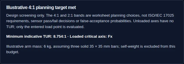
Actual worksheet result banner captured on November 4, 2026, using the initial teaching inputs: Fx=Fy=200 N, Fz=500 N, Mx=My=Mz=15 N·m, Lx=Ly=250 mm, Lz=100 mm, alignment half-range 0.35 mrad and reference standard u=0.01% of reading. Remaining inputs are the tool defaults. This records software execution with illustrative assumptions; it is not a physical calibration, customer result or evidence of equipment performance.
Example 1: Thermal material tradeoff (illustrative)
Premise: For the 100 N, 250 mm moment example above, compare assumed aluminum α=23.4 ppm/K with Invar α=1.2 ppm/K over ±2 K. The same ±20 µm rectangular location tolerance and u(F)=0.010 N apply.
Calculation / Process: Invar thermal half-range is 0.6 µm. Standard arm u is sqrt((20/√3)²+(0.6/√3)²)=11.55 µm; its geometry moment contribution is 0.001155 N·m.
Interpretation / Next Step: The two-term k=2 subtotal changes from 0.00567 N·m to 0.00551 N·m. Location and reference uncertainty dominate; changing material alone gives only a small improvement. Obtain actual CTE and geometry evidence before spending on Invar.
Example 2: A complete uncertainty allowance (illustrative)
Premise: For one 1000 N full-scale force channel with tolerance ±0.2% FS, the tolerance half-width is 2 N. Assume independent standard components: reference 0.10 N, alignment 0.20 N, compliance 0.05 N and residual transfer 0.03 N.
Interpretation / Next Step: This subtotal meets the worksheet planning target. Adding omitted sensor repeatability u=0.20 N raises U to 0.6112 N and lowers the ratio to 3.27. A favorable fixture subtotal is insufficient for accepting a sensor.
Example 3: Missing gravity and a workable fallback (illustrative)
Premise: A deadweight fixture has mass and arm certificates, but the site gravity value and mass convention are missing. The tool cannot quantify the remaining reference bias.
Calculation / Process: Leave the correction confirmations off and calculate: the estimate is marked incomplete. Request site gravity, density and the mass-convention details, or use a force transfer standard with suitable certificate evidence.
Interpretation / Next Step: No certificate or pass/fail claim is issued. Retain the worksheet as a design memo, collect the missing references, then repeat the load/reversal protocol and agree the complete decision rule with the lab.
14. Frequently Asked Questions
Mechanical Design
Do I need Invar lever arms?
Not automatically. Compare thermal expansion with location, force reference and alignment contributions. Example 1 shows that location and reference uncertainty can dominate even after lowering CTE. The CTE values here are illustrative; verify the material and operating temperature range.
Can I use a rod end or a rigid clamp?
Possibly, if measured parasitic reactions fit the budget. Contact type alone cannot predict the residual wrench. Check reversal hysteresis, joint freedom, stiffness and mounting constraints. The calculator factors are sensitivity assumptions, not bearing specifications.
How do I choose frame stiffness?
Set an allowed angular or linear displacement, then use kθ=M/θ or k=F/δ with consistent units. For 500 N and 0.1 mm, k=5000 kN/m. Include force-offset moments and verify loaded geometry; no one stiffness threshold suits every rig.
Which effective arms does the tool use?
It assumes Mx uses Ly, My uses Lx and Mz uses max(Lx,Ly); Lz only affects the illustrative mass estimate. These are simplified independent channel envelopes, not a solved spatial load path. For an actual fixture, survey every signed coordinate and apply M=r×F.
Metrology Traceability
Does an F1 weight or Class 00 load cell guarantee a fixed uncertainty?
No. Use the certificate value, coverage factor, load range and conditions. Convert U to standard u=U/k and convert to percent of reading at the test point. Reference class labels alone do not establish the complete uncertainty of the applied force.
What does confirming gravity and buoyancy mean?
It states that these corrections were handled outside the tool and that residual contributions are included in reference u. The tool does not calculate g or density. Unconfirmed corrections leave the estimate incomplete rather than substituting a generic bias.
What if my certificate states uncertainty in newtons or percent of full scale?
Convert at each test load. For example U=0.2 N, k=2 at F=100 N gives standard u=0.1 N, or 0.1% of reading. An FS-based percentage cannot be used unchanged as a reading-based percentage. Use a point-specific certificate value.
Which primary sources support this method?
JCGM 100 supplies uncertainty propagation principles; ILAC-G8 and JCGM 106 explain decision rules and risk. OIML R111 addresses mass standards. ComTraForce provides multicomponent and dynamic metrology context. The references below are linked directly and reviewed on November 4, 2026.
Error Budget & TUR
Does TUR ≥4:1 prove ISO/IEC 17025 compliance?
No. The 4:1 band here is a design planning choice. Accreditation, uncertainty and a statement of conformity require evidence beyond a ratio. ILAC-G8 explains documenting and agreeing the decision rule. No fixed false-acceptance probability can be inferred from this tool.
What happens at zero load or above full scale?
All-zero loads return an input error. An individual unloaded channel shows its estimated receiving-channel effects but no TUR. Per-axis loads above the entered full scale are rejected. Passing those checks does not verify the manufacturer combined-load envelope.
Does k=2 always mean 95% coverage?
No. It is an assumed coverage factor here. Coverage depends on distributions and effective degrees of freedom. A lab must evaluate whether that approximation is justified. The worksheet assumes independent components and does not include covariance.
How is the contribution chart calculated?
Only the loaded axis with the minimum indicative TUR is used. Each component variance is divided by that axis total variance. Force variances in N² are never added to moment variances in (N·m)². Unmodeled effects are absent from the chart.
Commissioning & Maintenance
Can a fixed-payload gravity tumble calibrate all six components?
No. For fixed r, M=[r]×F, so gravity-generated wrenches have at most three independent inputs. With an on-axis center of mass, Mz is always zero. Change offsets or apply independent couples to check missing moment modes; validate the robot frame convention before use.
Are 27 loading points enough for six-axis calibration?
It depends on rank and the model. A three-level, six-factor full factorial has 729 points; 27 points describes three factors. Selected designs can use fewer points, but must demonstrate rank, conditioning, repeats and independent validation. There is no automatic condition number from point count.
How long should I soak a thermal fixture?
Define measured stability and gradient criteria for the assembly and uncertainty budget. A fixed 45- or 60-minute soak is not established here. Record temperatures at the sensor and arm and verify drift before loading. Static results do not establish dynamic frequency response.
Can I request a fixture engineering review?
Send the design memo, sensor ranges, load-point drawing and reference certificates through the inquiry form. Availability, scope, deliverables and any accredited calibration must be confirmed separately. This page does not establish a supplied fixture product, certified performance or medical approval.
15. Sources, Review Date and Limitations
Prepared and reviewed by HexaForce Metrology & Robotics. Repository record created ; public publication date is unverified. Review again by May 4, 2027, or sooner if the cited standards change.
Standards and metrology review: . Source scope was checked against JCGM 100, ILAC-G8, JCGM 106, OIML R111 and the ComTraForce final report. Worksheet thresholds and residual coefficients are illustrative assumptions, not prescribed standard limits.
Sections 4–6 explain standard uncertainty, sensitivity coefficients, covariance and coverage factors. This worksheet assumes independent contributions; it is not a complete application of the GUM.
Explains how conformance risk depends on the measurement model, results, distributions and decision rule. No fixed false-pass probability is claimed here.
Mass class requirements and nominal mass matter. A class label is not a universal force uncertainty; use certificate values and gravity/buoyancy corrections.
Research on force traceability, static/continuous/dynamic measurements, multicomponent methods and temperature effects. It supplies context, not performance ratings for the illustrative rigs on this page.
Material CTEs and effective friction/transfer factors are illustrative assumptions without a verified grade, bearing or rig dataset. The static worksheet excludes covariance, sensor response, arm self-weight and actual load-point geometry. Verify these before making a calibration decision.
Need Custom 6-Axis Calibration Fixtures or Rig Engineering?
Share the load envelope, mounting drawing, reference certificates and design estimate for an engineering discussion. Scope, availability and any accredited calibration service must be confirmed separately.